Section 4 Downstream Visualizations
Description: This pipeline performs downstream visualizations, including volcano plot, heatmap, and box plots.
Project Initialization:
#Sets the working directory and creates subfolders for organizing outputs.
mypath= "C:/Users/USER/Documents/Github/CRC_project/"
dir.create("output")
dir.create("plots")
dir.create("input")
#Load libraries
library(tibble)
library(plyr)
library(dplyr)
library(tidyverse)
library(openxlsx)
library(cowplot)
library(ggplot2)
library(tibble)
library("RColorBrewer")
library("circlize")
library(ComplexHeatmap)
library(biomaRt)
library(dplyr)
library(plyr)
library(fields)
library(tidyr)
library(RColorBrewer)
library(viridis)
library(ggplot2)
library(ggrepel)#load data
data= read.csv(paste0(mypath,"input/data_for_downstream.csv"))
data = data %>% column_to_rownames(colnames(data)[1]) %>% dplyr::select(-1)
de= read.csv(paste0(mypath,"output/DE_sig.csv"))
de=de |> filter(abs(logFC) >= log2(3))
output_dir= paste0(mypath, "output/")
# set group distribution for samples
group_dist= gsub("_.*", "", colnames(data))
print(group_dist)## [1] "CRC" "CRC" "CRC" "CRC" "CRC" "CRC" "CRC" "CRC" "CRC" "Ctrl"
## [11] "Ctrl" "Ctrl" "Ctrl" "Ctrl" "Ctrl" "Ctrl" "Ctrl" "Ctrl" "Ctrl"group_levels= unique(group_dist)
group_colors <- c("#fc8d62", "#66c2a5")
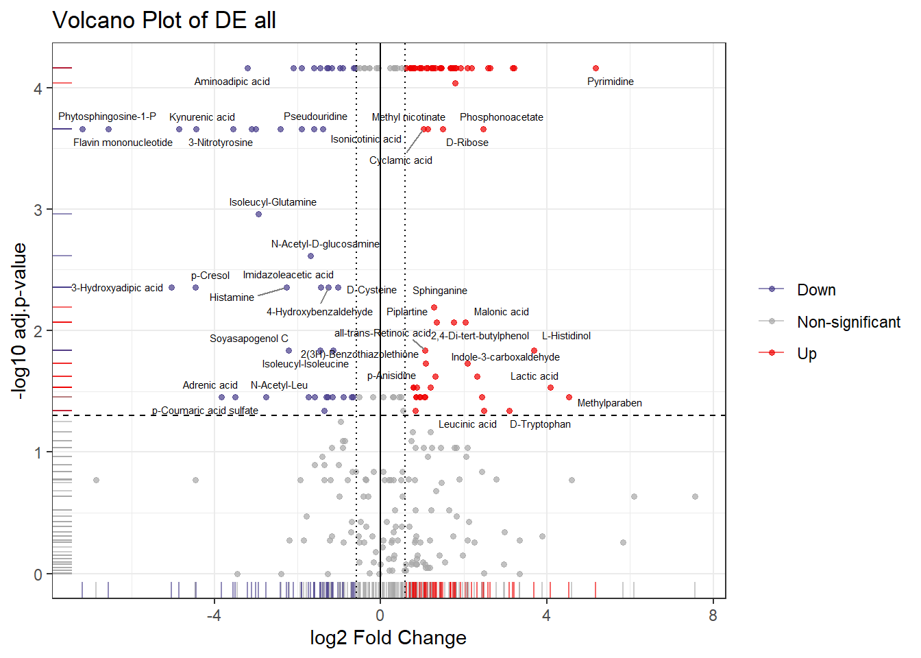
names(group_colors) <- group_levels4.1 Volcano Plot
plot_volcano = function(file_path=NULL, df=NULL, name=NULL,
                        plot_dir = "plots", fc_threshold = 1.5) {

  if (!dir.exists(plot_dir)) dir.create(plot_dir, recursive = TRUE)
    # Read the DE result
  if(!is.null(file_path)){
    res <- read.csv(file_path)
    name <- gsub(".*_([[:alnum:] ]+)\\.csv$", "\\1", basename(file_path))
  }

  if(!is.null(df) & !is.null(name)){
    res= df
    name= name
  }
    res <- as.data.frame(res)
    colnames(res)[grepl("log",colnames(res) )]= "logFC"
    colnames(res)[grepl("adj|FDR",colnames(res) )]= "padj"
    res$padj[is.na(res$padj)]= res$pval[is.na(res$padj)]

    # Define direction
    res$Direction <- ifelse(res$padj <= 0.05 & res$logFC >= log2(fc_threshold), "Up",
                            ifelse(res$padj <= 0.05 & res$logFC <= -log2(fc_threshold), "Down",
                                                                             "Non-significant"))
    # Keep only labels for up or down expressed features
    res <- res %>% mutate(features = ifelse(Direction %in% c("Up", "Down"), X, ""))
    # Compute -log10(p-value)
    res$log10p <- -log10(res$padj)
    # Plot parameters
    xminma <- -3.5
    xmaxma <- 3.5

    # Generate the plot
    volcano <- ggplot(res, aes(x = logFC, y = log10p, color = Direction, label = features)) +
      geom_point(size = 1.2, alpha = 0.7) +
      geom_rug(alpha = 0.6) +
      scale_color_manual(values = c("Up" = "red2", "Down" = "darkslateblue", "Non-significant" = "grey66")) +
      xlab('log2 Fold Change') +
      ylab('-log10 adj.p-value') +
      #scale_x_continuous(limits = c(xminma, xmaxma)) +
      theme_bw() +
      theme(legend.title = element_blank()) +
      geom_vline(xintercept = c(-log2(fc_threshold), 0, log2(fc_threshold)), linetype = c("dotted", "solid", "dotted")) +
      geom_hline(yintercept = -log10(0.05), linetype = "dashed") +
      geom_text_repel(aes(label = features),
                      size = 2,
                      max.overlaps = 10,
                      segment.color = "grey50",
                      color = "black") +
      ggtitle(paste0("Volcano Plot of DE ", name))

    # Print and save
    print(volcano)
    ggsave(filename = paste0(plot_dir, "/Volcanoplot_", name, ".jpg"),
           plot = volcano,
           dpi = 600,
           width = 7,
           height = 4)
  }
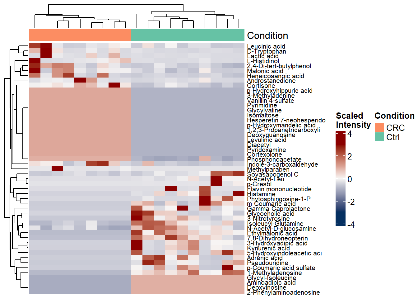
4.2 Heatmap Plot
plot_heatmap= function(data= NULL, de= NULL, group_dist, group_colors ){

    #you can use for loop for multiple groups DE files
    data_sub= data[row.names(data) %in% de$X, ]
    #data= data %>% dplyr::slice(1:50)
    #row.names= gsub("\\%.*", "", row.names(data))
    heat_data=  t(scale(t(data_sub)))  # center row wise
    rownames(heat_data)=  substr(rownames(heat_data), 1, 25)

    ta <- HeatmapAnnotation(
      Condition = group_dist,
      col = list(
        Condition = group_colors

      ),
      annotation_height = unit(10, "mm")
    )

    #palt=  colorRampPalette(c("blue4", "black", "#8B0000"))(256)
    #palt= colorRampPalette(viridis(n = 8))(200)
    palt= colorRamp2(c(-3, 0, 3), c("#053061", "#F7F5F4", "darkred"))

    heatmap  <- Heatmap(
      matrix = as.matrix(heat_data),
      name = "Normalized Intensity",
      col =palt ,#' ## ' #' ## #' ## matlab::jet.colors(200),
      show_row_names = TRUE,
      cluster_rows = TRUE,
      cluster_columns = TRUE,
      show_column_names = FALSE,
      row_names_gp = gpar(fontsize = 8),
      top_annotation  = ta,
      heatmap_legend_param = list(
        title= "Scaled\nIntensity",
        title_gp = gpar(fontsize = 10, fontface = "bold"),
        labels_gp = gpar(fontsize = 10),
        legend_height = unit(4, "cm"),
        legend_width = unit(.5, "cm")
      )
    )
    print(heatmap)
    png("plots/heatmap.png",width = 4000, height = 5000, res = 600)
    draw(heatmap, annotation_legend_side = "right", heatmap_legend_side = "right") #"right"
    dev.off()

}
## png
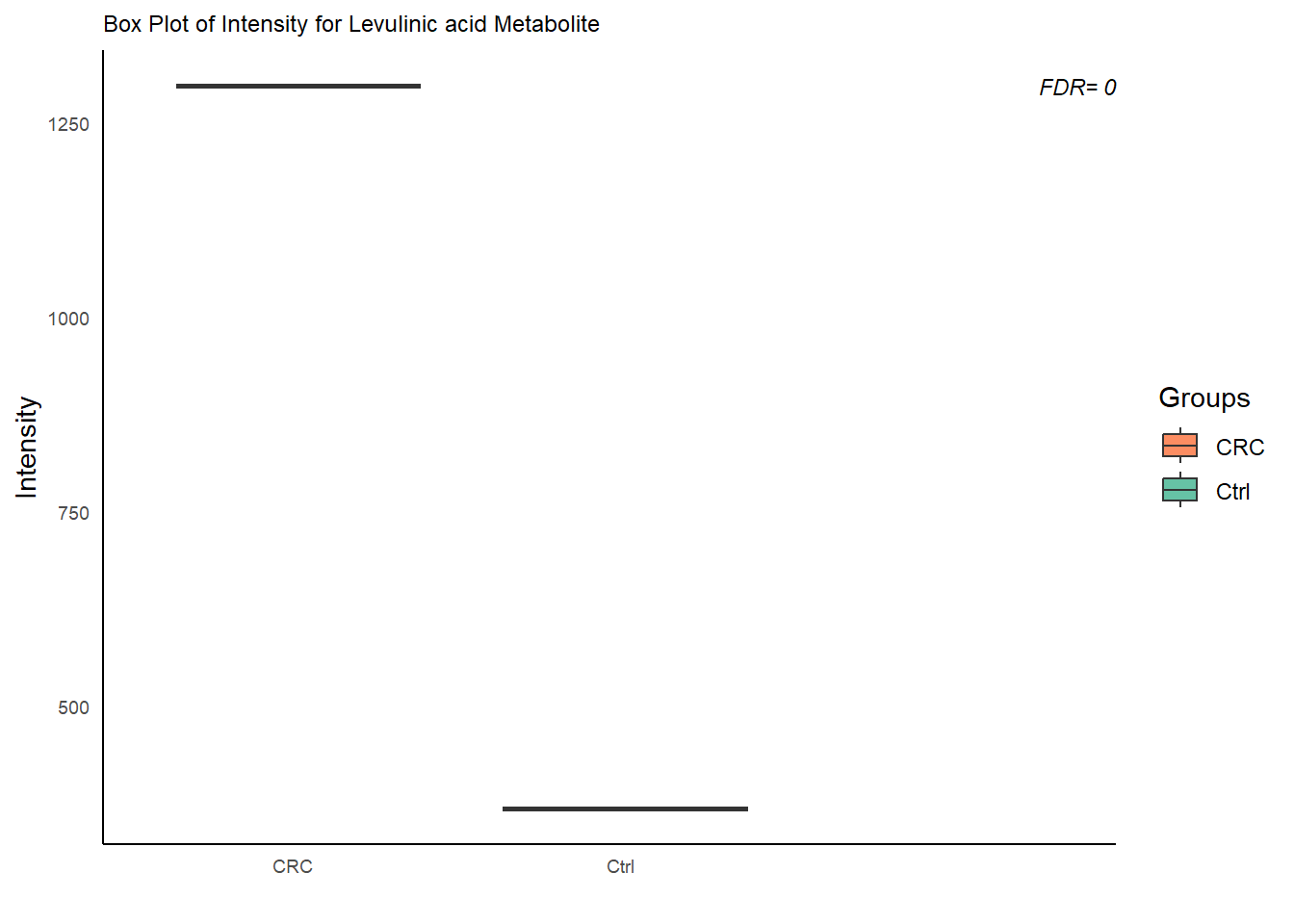
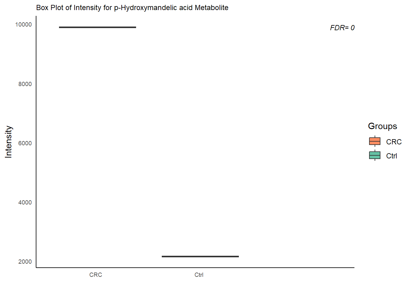
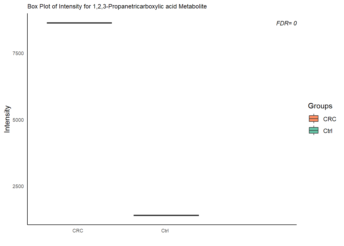
## 24.3 Box Plots
# Loop over DE features
plot_box= function( data=NULL, de= NULL, group_dist){

    data= data[row.names(data) %in% de$X, ]
    data.t= t(data)
    de <- as.data.frame(de)
    colnames(de)[grepl("log",colnames(de) )]= "logFC"
    colnames(de)[grepl("adj|FDR",colnames(de) )]= "padj"
    de$padj[is.na(de$padj)]= de$pval[is.na(de$padj)]

for (m in colnames(data.t)) {
    # Subset data
    data.box = data.frame(
            value= data.t[, m],
            group= group_dist)

    FDR= de$padj[de$X== m]
    quartile.t= quantile(  data.box$value, 0.90)

    p= ggplot(data.box , aes(x = group , y = value , fill= group)) +
      geom_boxplot() +
      scale_fill_manual(values = group_colors )+
      labs(title = paste0("Box Plot of Intensity for ", m, " Metabolite"), x = "",
           y = "Intensity",
           fill= "Groups")+
      annotate("text",
               x = 3.5,
               y =  quartile.t,
               label = paste0( "FDR= " , round(FDR, 2)) ,
               size = 3, fontface = "italic", hjust = 1) +
      theme_minimal()+
      theme(
        axis.text.x = element_text(angle = 0, hjust = .65, size = 7),
        axis.text.y = element_text(size = 7),
        plot.title = element_text(size = 9),
        axis.line = element_line(color = "black"),
        panel.grid = element_blank(),
        axis.ticks = element_blank(),
        panel.border = element_blank())

    print(p)
    ggsave(paste0("plots/boxplot_" , m, ".png"), p, width=5, height =4, dpi=600)

  }
}
## R version 4.4.1 (2024-06-14 ucrt)
## Platform: x86_64-w64-mingw32/x64
## Running under: Windows 10 x64 (build 19045)
##
## Matrix products: default
##
##
## locale:
## [1] LC_COLLATE=English_United States.utf8
## [2] LC_CTYPE=English_United States.utf8
## [3] LC_MONETARY=English_United States.utf8
## [4] LC_NUMERIC=C
## [5] LC_TIME=English_United States.utf8
##
## time zone: Africa/Cairo
## tzcode source: internal
##
## attached base packages:
## [1] grid      stats     graphics  grDevices utils     datasets  methods
## [8] base
##
## other attached packages:
##  [1] ggrepel_0.9.6         viridis_0.6.5         fields_16.2
##  [4] viridisLite_0.4.2     spam_2.10-0           biomaRt_2.61.2
##  [7] ComplexHeatmap_2.21.0 circlize_0.4.16       RColorBrewer_1.1-3
## [10] memoise_2.0.1         caret_6.0-94          lattice_0.22-6
## [13] pls_2.8-3             Rserve_1.8-13         MetaboAnalystR_3.2.0
## [16] cowplot_1.1.3         DT_0.33               openxlsx_4.2.6.1
## [19] lubridate_1.9.3       forcats_1.0.0         stringr_1.5.1
## [22] purrr_1.0.2           readr_2.1.5           tidyr_1.3.1
## [25] ggplot2_3.5.1         tidyverse_2.0.0       dplyr_1.1.4
## [28] plyr_1.8.9            tibble_3.2.1
##
## loaded via a namespace (and not attached):
##   [1] splines_4.4.1           filelock_1.0.3          bitops_1.0-7
##   [4] hardhat_1.4.0           pROC_1.18.5             rpart_4.1.23
##   [7] httr2_1.0.2             lifecycle_1.0.4         edgeR_4.3.5
##  [10] doParallel_1.0.17       globals_0.16.3          MASS_7.3-60.2
##  [13] scrime_1.3.5            crosstalk_1.2.1         magrittr_2.0.3
##  [16] limma_3.61.5            plotly_4.10.4           sass_0.4.9
##  [19] rmarkdown_2.27          jquerylib_0.1.4         yaml_2.3.10
##  [22] zip_2.3.1               DBI_1.2.3               maps_3.4.2
##  [25] zlibbioc_1.50.0         BiocGenerics_0.52.0     nnet_7.3-19
##  [28] rappdirs_0.3.3          ipred_0.9-15            GenomeInfoDbData_1.2.12
##  [31] lava_1.8.0              IRanges_2.38.1          S4Vectors_0.42.1
##  [34] listenv_0.9.1           ellipse_0.5.0           parallelly_1.38.0
##  [37] codetools_0.2-20        xml2_1.3.6              RApiSerialize_0.1.3
##  [40] tidyselect_1.2.1        shape_1.4.6.1           UCSC.utils_1.1.0
##  [43] farver_2.1.2            BiocFileCache_2.13.0    matrixStats_1.3.0
##  [46] stats4_4.4.1            jsonlite_1.8.8          GetoptLong_1.0.5
##  [49] multtest_2.61.0         e1071_1.7-14            survival_3.6-4
##  [52] iterators_1.0.14        systemfonts_1.2.3       foreach_1.5.2
##  [55] progress_1.2.3          tools_4.4.1             ragg_1.3.2
##  [58] Rcpp_1.0.13             glue_1.7.0              gridExtra_2.3
##  [61] prodlim_2024.06.25      xfun_0.46               GenomeInfoDb_1.41.1
##  [64] crmn_0.0.21             withr_3.0.0             fastmap_1.2.0
##  [67] caTools_1.18.2          digest_0.6.36           timechange_0.3.0
##  [70] R6_2.5.1                textshaping_0.4.0       colorspace_2.1-1
##  [73] Cairo_1.6-2             gtools_3.9.5            RSQLite_2.3.7
##  [76] generics_0.1.3          data.table_1.15.4       recipes_1.1.0
##  [79] class_7.3-22            prettyunits_1.2.0       httr_1.4.7
##  [82] htmlwidgets_1.6.4       ModelMetrics_1.2.2.2    pkgconfig_2.0.3
##  [85] gtable_0.3.5            timeDate_4032.109       blob_1.2.4
##  [88] siggenes_1.79.0         impute_1.79.0           XVector_0.44.0
##  [91] htmltools_0.5.8.1       dotCall64_1.1-1         bookdown_0.40
##  [94] fgsea_1.31.0            clue_0.3-65             scales_1.3.0
##  [97] Biobase_2.64.0          png_0.1-8               gower_1.0.1
## [100] knitr_1.48              rstudioapi_0.16.0       tzdb_0.4.0
## [103] reshape2_1.4.4          rjson_0.2.21            curl_5.2.1
## [106] nlme_3.1-164            proxy_0.4-27            cachem_1.1.0
## [109] GlobalOptions_0.1.2     KernSmooth_2.23-24      parallel_4.4.1
## [112] AnnotationDbi_1.67.0    pillar_1.11.0           vctrs_0.6.5
## [115] gplots_3.1.3.1          pcaMethods_1.97.0       stringfish_0.16.0
## [118] dbplyr_2.5.0            cluster_2.1.6           evaluate_0.24.0
## [121] magick_2.8.4            cli_3.6.3               locfit_1.5-9.10
## [124] compiler_4.4.1          rlang_1.1.4             crayon_1.5.3
## [127] future.apply_1.11.2     labeling_0.4.3          stringi_1.8.4
## [130] BiocParallel_1.39.0     munsell_0.5.1           Biostrings_2.72.1
## [133] lazyeval_0.2.2          Matrix_1.7-0            hms_1.1.3
## [136] glasso_1.11             bit64_4.0.5             future_1.33.2
## [139] KEGGREST_1.45.1         statmod_1.5.0           highr_0.11
## [142] qs_0.26.3               igraph_2.0.3            RcppParallel_5.1.8
## [145] bslib_0.8.0             fastmatch_1.1-4         bit_4.0.5