Section 2 Dimensionality Reduction Techniques
Description: This pipeline performs variuos dimensionality reduction techniques: PCA and PLS-DA and sPLS-DA- using Metaboanalyst R package.
Project Initialization:
mypath= "C:/Users/USER/Documents/Github/CRC_project/"
# Uncomment the following commands
dir.create("output")
dir.create("plots")
dir.create("input")
#Load libraries
library(tibble)
library(plyr)
library(dplyr)
library(tidyverse)
library(openxlsx)
library(cowplot)
library(ggplot2)
library("MetaboAnalystR")
library(DT)
#BiocManager::install("DT")#load data
data= read.csv(paste0(mypath,"input/data_for_downstream.csv"))
data = data |> column_to_rownames(colnames(data)[1]) 2.1 Input data Preparation for Metaboanalyst
#Specify the group pattern in your samples and add it as the first row in the sheet.
group_dist= gsub("_.*", "", colnames(data))
group_levels= unique(group_dist)
print(group_dist)
## [1] "CRC" "CRC" "CRC" "CRC" "CRC" "CRC" "CRC" "CRC" "CRC" "CRC"
## [11] "Ctrl" "Ctrl" "Ctrl" "Ctrl" "Ctrl" "Ctrl" "Ctrl" "Ctrl" "Ctrl" "Ctrl"data_formatted= rbind(group_dist, data)
datatable(data_formatted, options = list(scrollX=TRUE, scrollY="600px", autoWidth = TRUE))## Starting Rserve...
## "C:\Users\USER\AppData\Local\R\WIN-LI~1\4.4\Rserve\libs\x64\Rserve.exe" --no-save
## [1] "MetaboAnalyst R objects initialized ..."mSet<-Read.TextData(mSet, paste0(mypath,"output/for_metaboanalyst.csv"), "colu", "disc")
mSet<-SanityCheckData(mSet)## [1] "Successfully passed sanity check!"
## [2] "Samples are not paired."
## [3] "2 groups were detected in samples."
## [4] "Only English letters, numbers, underscore, hyphen and forward slash (/) are allowed."
## [5] "<font color=\"orange\">Other special characters or punctuations (if any) will be stripped off.</font>"
## [6] "All data values are numeric."
## [7] "A total of 0 (0%) missing values were detected."
## [8] "<u>By default, missing values will be replaced by 1/5 of min positive values of their corresponding variables</u>"
## [9] "Click the <b>Proceed</b> button if you accept the default practice;"
## [10] "Or click the <b>Missing Values</b> button to use other methods."2.2 PCA
Principal Component Analysis (PCA) is a dimensionality reduction technique used to explore patterns in high-dimensional data. It transforms the original variables into a smaller set of uncorrelated variables called principal components, which capture the maximum variance in the data. PCA is often used for data visualization, outlier detection, and identifying natural clusters or trends without any prior knowledge of group labels and so it is unsupervised!
mSet<-PCA.Anal(mSet)
mSet<-PlotPCA2DScore(mSet, paste0(mypath,"plots/PCA_2D"), "png", 150, width=NA, 1,2,0.95,0,0)
PCA_data <- mSet$analSet$pca$x
write.csv(PCA_data, paste0(mypath,"output/pca_score.csv") , row.names = TRUE)
PCA plot
# Load PCA data with samples as row names
PCA_data <- read.csv(paste0(mypath, "output/pca_score.csv"), row.names = 1)

# Calculate variance explained by each principal component
vars <- apply(PCA_data, 2, var)
PC1_var <- round((var(PCA_data$PC1) / sum(vars)) * 100, 1)
PC2_var <- round((var(PCA_data$PC2) / sum(vars)) * 100, 1)
PC3_var <- round((var(PCA_data$PC3) / sum(vars)) * 100, 1)

# Add group metadata
PCA_data$group = group_dist
group_colors <- c("#fc8d62", "#66c2a5")
names(group_colors) <- group_levels

pca_plot= ggplot(PCA_data, aes(x = PC1, y = PC2, colour = group)) +
      stat_ellipse(aes(fill = group), level = 0.95, geom = "polygon", alpha = 0.1, colour = NA) +
      geom_point(aes(fill = group), alpha = 0.7, shape = 21, size = 4,
                 colour = "black", stroke = 1.5) +
      scale_fill_manual(values = group_colors) +
      scale_color_manual(values = group_colors) +
      labs(color = "Groups", fill = "Groups") +
      xlab(paste0("PC1 (", PC1_var, "%)")) +
      ylab(paste0("PC2 (", PC2_var, "%)")) +
      theme(
            #legend.background = element_rect(size = 0.5, linetype = "solid", colour = "black"),
            legend.title = element_text(face = "bold", size = 14),
            legend.position = "right",
            text = element_text(size = 16, face = "bold")) +
      theme( plot.background = element_rect(fill = "white", color = NA),
             panel.background = element_rect(fill = "white", color = NA),
             panel.grid = element_blank(),
             axis.line = element_line(color = "black"),
             axis.ticks = element_line(color = "black"),
             text = element_text(face = "bold"),
             plot.title = element_text(hjust = 0.5))

print(pca_plot)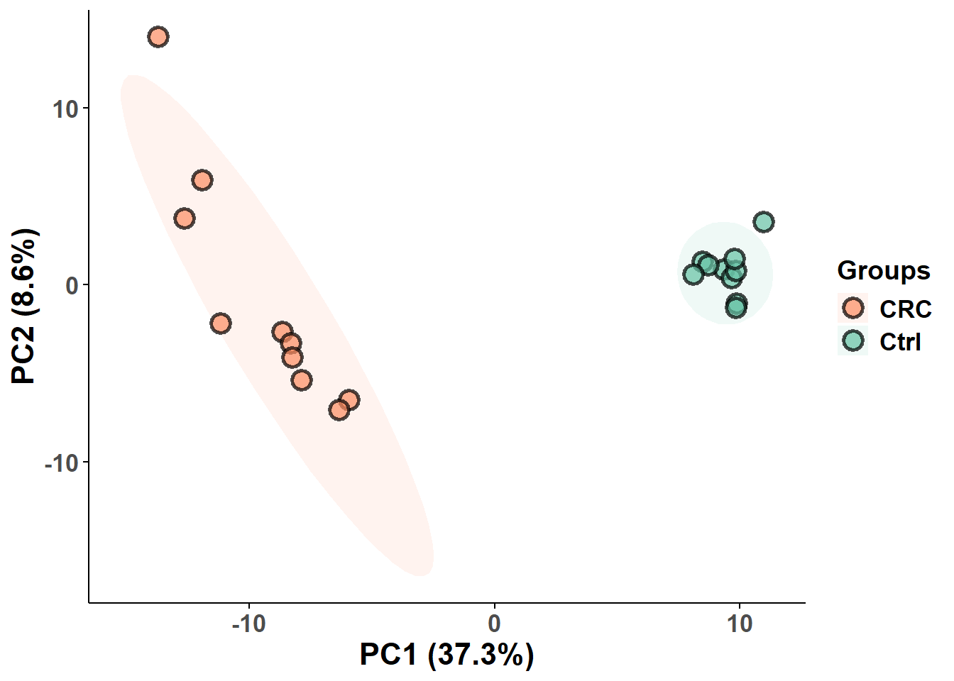
2.3 PLS-DA
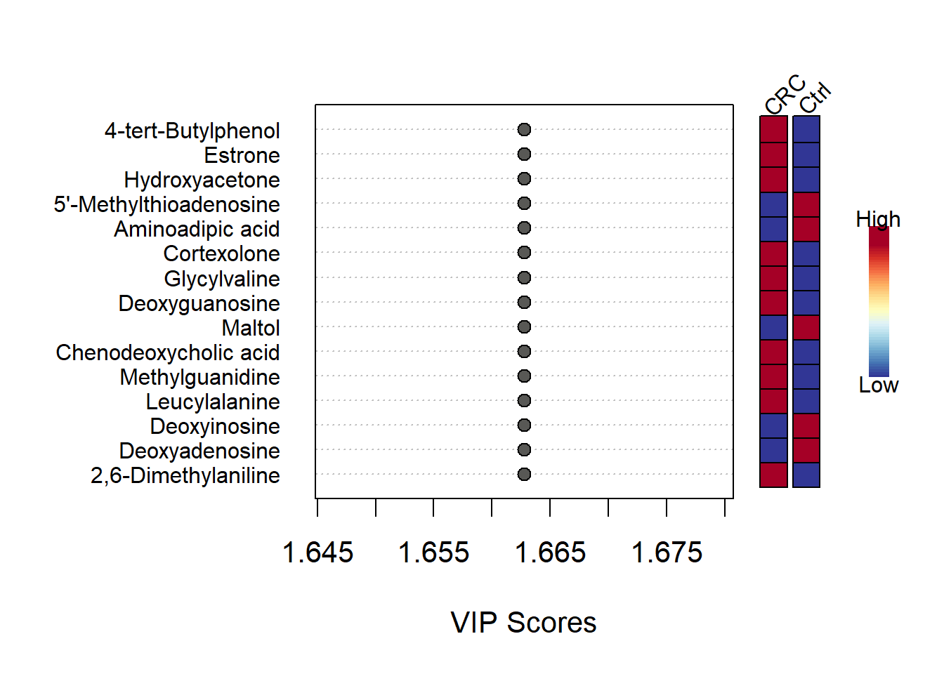
Partial Least Squares Discriminant Analysis (PLS-DA) is a supervised method that combines PLS regression with classification. PLS-DA models the relationship between predictors (e.g., gene or metabolite expression) and a categorical outcome (e.g., disease status), maximizing the covariance between them. And so It does find directions in the data that best separate predefined groups or classes.
library(pls)
# call adjusted function for VIP plot
source("C:/Users/USER/Documents/Rscripts/All_Functions/plot_vip.R")
mSet<-PLSR.Anal(mSet, reg=TRUE)

mSet<-PlotPLSPairSummary(mSet, paste0(mypath, "plots/pls_pair"), "png", 72, width=NA, 5)
mSet<-PlotPLS2DScore(mSet, paste0(mypath,"plots/pls_score2d"), "png", 72, width=NA, 1,2,0.95,0,0)
mSet<-PlotPLS3DScoreImg(mSet, paste0(mypath,"plots/pls_score3d"), "png", 72, width=NA, 1,2,3, 40)
mSet<-PlotPLSLoading(mSet, paste0(mypath,"plots/pls_loading"), "png", 72, width=NA, 1, 2);
mSet<-PLSDA.CV(mSet, "T",5, "Q2")
mSet<-PlotPLS.Classification(mSet, paste0(mypath,"plots/pls_cv"), "png", 72, width=NA)
mSet<-PlotPLS.Imp(mSet, paste0(mypath,"plots/pls_imp"), "png", 72, width=7, "vip", "Comp. 1", 15,  FALSE)
mSet<-PLSDA.Permut(mSet, 100, "accu")
## [1] "performing 100 permutations ..."
## [1] "Empirical p value: p = 1 (100/100)"VIP plot for displaying top features discriminating the two groups
## $mar
## [1] 5 9 3 6
# Save
png(paste0(mypath,"plots/vip_plot2.png"), unit = "in",res = 600, width = 7, height = 7)
Plotvip(mSetObj = mSet,feat.num=15, color.BW =FALSE)
dev.off()## png
## 22.4 splsda
Sparse PLS-DA (sPLS-DA) extends PLS-DA by introducing variable selection through sparsity constraints. It separates classes while identifying a minimal set of discriminative features.
# # Perform sPLS-DA analysis
# mSet<-SPLSR.Anal(mSet, 1, 1, "same", "Mfold")
# # Plot sPLS-DA overview
# mSet<-PlotSPLSPairSummary(mSet, paste0(mypath,"plots/spls_pair"), format = "png", dpi=72, width=NA, 5)
# # Create 2D sPLS-DA Score Plot
# mSet<-PlotSPLS2DScore(mSet, paste0(mypath,"plots/spls_score2d"), format = "png", dpi=72, width=NA, 1, 2, 0.95, 1, 0)
# # Create 3D sPLS-DA Score Plot
# mSet<-PlotSPLS3DScoreImg(mSet, paste0(mypath,"plots/spls_score3d"), format = "png", 72, width=NA, 1, 2, 3, 40)
# # Create sPLS-DA loadings plot
# mSet<-PlotSPLSLoading(mSet, paste0(mypath,"plots/spls_loading"), format = "png", dpi=72, width=NA, 1,"overview")
# # Perform cross-validation and plot sPLS-DA classification
# mSet<-PlotSPLSDA.Classification(mSet, paste0(mypath,"plots/spls_cv"), format = "png", dpi=72, width=NA)
## R version 4.4.1 (2024-06-14 ucrt)
## Platform: x86_64-w64-mingw32/x64
## Running under: Windows 10 x64 (build 19045)
##
## Matrix products: default
##
##
## locale:
## [1] LC_COLLATE=English_United States.utf8
## [2] LC_CTYPE=English_United States.utf8
## [3] LC_MONETARY=English_United States.utf8
## [4] LC_NUMERIC=C
## [5] LC_TIME=English_United States.utf8
##
## time zone: Africa/Cairo
## tzcode source: internal
##
## attached base packages:
## [1] stats graphics grDevices utils datasets methods base
##
## other attached packages:
## [1] caret_6.0-94 lattice_0.22-6 pls_2.8-3
## [4] Rserve_1.8-13 MetaboAnalystR_3.2.0 cowplot_1.1.3
## [7] DT_0.33 openxlsx_4.2.6.1 lubridate_1.9.3
## [10] forcats_1.0.0 stringr_1.5.1 purrr_1.0.2
## [13] readr_2.1.5 tidyr_1.3.1 ggplot2_3.5.1
## [16] tidyverse_2.0.0 dplyr_1.1.4 plyr_1.8.9
## [19] tibble_3.2.1
##
## loaded via a namespace (and not attached):
## [1] RColorBrewer_1.1-3 rstudioapi_0.16.0 jsonlite_1.8.8
## [4] magrittr_2.0.3 farver_2.1.2 rmarkdown_2.27
## [7] ragg_1.3.2 vctrs_0.6.5 multtest_2.61.0
## [10] memoise_2.0.1 Cairo_1.6-2 htmltools_0.5.8.1
## [13] pROC_1.18.5 sass_0.4.9 parallelly_1.38.0
## [16] KernSmooth_2.23-24 bslib_0.8.0 htmlwidgets_1.6.4
## [19] impute_1.79.0 plotly_4.10.4 cachem_1.1.0
## [22] igraph_2.0.3 lifecycle_1.0.4 iterators_1.0.14
## [25] pkgconfig_2.0.3 Matrix_1.7-0 R6_2.5.1
## [28] fastmap_1.2.0 future_1.33.2 digest_0.6.36
## [31] pcaMethods_1.97.0 colorspace_2.1-1 siggenes_1.79.0
## [34] textshaping_0.4.0 crosstalk_1.2.1 ellipse_0.5.0
## [37] RSQLite_2.3.7 labeling_0.4.3 timechange_0.3.0
## [40] httr_1.4.7 compiler_4.4.1 proxy_0.4-27
## [43] bit64_4.0.5 withr_3.0.0 glasso_1.11
## [46] BiocParallel_1.39.0 DBI_1.2.3 qs_0.26.3
## [49] highr_0.11 gplots_3.1.3.1 MASS_7.3-60.2
## [52] lava_1.8.0 gtools_3.9.5 caTools_1.18.2
## [55] ModelMetrics_1.2.2.2 tools_4.4.1 zip_2.3.1
## [58] future.apply_1.11.2 nnet_7.3-19 glue_1.7.0
## [61] nlme_3.1-164 grid_4.4.1 reshape2_1.4.4
## [64] fgsea_1.31.0 generics_0.1.3 recipes_1.1.0
## [67] gtable_0.3.5 tzdb_0.4.0 class_7.3-22
## [70] data.table_1.15.4 RApiSerialize_0.1.3 hms_1.1.3
## [73] stringfish_0.16.0 BiocGenerics_0.52.0 foreach_1.5.2
## [76] pillar_1.11.0 limma_3.61.5 splines_4.4.1
## [79] survival_3.6-4 bit_4.0.5 tidyselect_1.2.1
## [82] locfit_1.5-9.10 knitr_1.48 bookdown_0.40
## [85] edgeR_4.3.5 stats4_4.4.1 xfun_0.46
## [88] Biobase_2.64.0 scrime_1.3.5 statmod_1.5.0
## [91] hardhat_1.4.0 timeDate_4032.109 stringi_1.8.4
## [94] lazyeval_0.2.2 yaml_2.3.10 evaluate_0.24.0
## [97] codetools_0.2-20 crmn_0.0.21 cli_3.6.3
## [100] RcppParallel_5.1.8 rpart_4.1.23 systemfonts_1.2.3
## [103] munsell_0.5.1 jquerylib_0.1.4 Rcpp_1.0.13
## [106] globals_0.16.3 parallel_4.4.1 gower_1.0.1
## [109] blob_1.2.4 bitops_1.0-7 listenv_0.9.1
## [112] viridisLite_0.4.2 ipred_0.9-15 e1071_1.7-14
## [115] scales_1.3.0 prodlim_2024.06.25 rlang_1.1.4
## [118] fastmatch_1.1-4